Note
Click here to download the full example code
Contributions of up- and downgoing TM- and TE-modes
This is an example for the add-on tmtemod. The example is taken from the
CSEM-book by Ziolkowski and Slob, 2019. Have a look at the CSEM-book repository
on empymod/csem-ziolkowski-and-slob for many more examples.
Reference
- Ziolkowski, A., and E. Slob, 2019, Introduction to Controlled-Source Electromagnetic Methods: Cambridge University Press; ISBN 9781107058620.
import empymod
import numpy as np
import matplotlib.pyplot as plt
plt.style.use('ggplot')
Model parameters
# Offsets
x = np.linspace(10, 1.5e4, 128)

# Resistivity model
rtg = [2e14, 1/3, 1, 70, 1]  # With target
rhs = [2e14, 1/3, 1, 1, 1]   # Half-space

# Common model parameters (deep sea parameters)
model = {
    'src': [0, 0, 975],              # Source location
    'rec': [x, x*0, 1000],           # Receiver location
    'depth': [0, 1000, 2000, 2040],  # 1 km water, target 40 m thick 1 km below
    'freqtime': 0.5,                 # Frequencies
    'verb': 1,                       # Verbosity
}
Computation
target = empymod.dipole(res=rtg, **model)
tgTM, tgTE = empymod.tmtemod.dipole(res=rtg, **model)

# Without reservoir
notarg = empymod.dipole(res=rhs, **model)
ntTM, ntTE = empymod.tmtemod.dipole(res=rhs, **model)
Figure 1
Plot all reflected contributions (without direct field), for the models with and without a reservoir.
plt.figure(figsize=(10, 4))

# 1st subplot
ax1 = plt.subplot(121)
plt.semilogy(x/1000, np.abs(tgTE[0]), 'C0-.')
plt.semilogy(x/1000, np.abs(ntTE[0]), 'k-.', label='TE$^{--}$')
plt.semilogy(x/1000, np.abs(tgTE[2]), 'C0-')
plt.semilogy(x/1000, np.abs(ntTE[2]), 'k-', label='TE$^{+-}$')
plt.semilogy(x/1000, np.abs(tgTE[1]), 'C0--')
plt.semilogy(x/1000, np.abs(ntTE[1]), 'k--', label='TE$^{-+}$')
plt.semilogy(x/1000, np.abs(tgTE[3]), 'C0:')
plt.semilogy(x/1000, np.abs(ntTE[3]), 'k:', label='TE$^{++}$')
plt.semilogy(-1, 1, 'k-', label='No target')  # Dummy entries for labels
plt.semilogy(-1, 1, 'C0-', label='Target')     # "
plt.legend()
plt.xlabel('Offset (km)')
plt.ylabel('Electric field amplitude (V/m)')
plt.xlim([0, 15])

# 2nd subplot
plt.subplot(122, sharey=ax1)
plt.semilogy(x/1000, np.abs(tgTM[0]), 'C0-.')
plt.semilogy(x/1000, np.abs(ntTM[0]), 'k-.', label='TM$^{--}$')
plt.semilogy(x/1000, np.abs(tgTM[2]), 'C0-')
plt.semilogy(x/1000, np.abs(ntTM[2]), 'k-', label='TM$^{+-}$')
plt.semilogy(x/1000, np.abs(tgTM[1]), 'C0--')
plt.semilogy(x/1000, np.abs(ntTM[1]), 'k--', label='TM$^{-+}$')
plt.semilogy(x/1000, np.abs(tgTM[3]), 'C0:')
plt.semilogy(x/1000, np.abs(ntTM[3]), 'k:', label='TM$^{++}$')
plt.semilogy(-1, 1, 'k-', label='No target')  # Dummy entries for labels
plt.semilogy(-1, 1, 'C0-', label='Target')     # "
plt.legend()
plt.xlabel('Offset (km)')
plt.ylim([1e-17, 1e-9])
plt.xlim([0, 15])

plt.show()
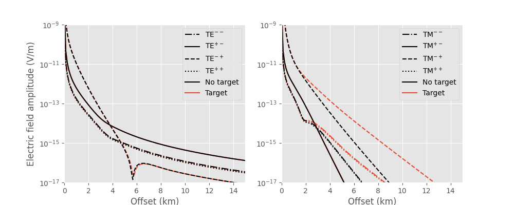
The result shows that mainly the TM-mode contributions are sensitive to the reservoir. For TM, all modes contribute significantly except $T^{+-}$, which is the field that travels upwards from the source and downwards to the receiver.
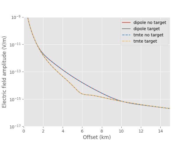
Figure 2
Finally we check if the result from empymod.dipole equals the sum of the
output of empymod.tmtemod.dipole.
plt.figure()

nt = ntTM[0]+ntTM[1]+ntTM[2]+ntTM[3]+ntTM[4]
nt += ntTE[0]+ntTE[1]+ntTE[2]+ntTE[3]+ntTE[4]
tg = tgTM[0]+tgTM[1]+tgTM[2]+tgTM[3]+tgTM[4]
tg += tgTE[0]+tgTE[1]+tgTE[2]+tgTE[3]+tgTE[4]

plt.semilogy(x/1000, np.abs(target), 'C0-', label='dipole no target')
plt.semilogy(x/1000, np.abs(notarg), 'C3-', label='dipole target')
plt.semilogy(x/1000, np.abs(tg), 'C1--', label='tmte no target')
plt.semilogy(x/1000, np.abs(nt), 'C4--', label='tmte target')
plt.legend()
plt.xlabel('Offset (km)')
plt.ylabel('Electric field amplitude (V/m)')
plt.ylim([1e-17, 1e-9])
plt.xlim([0, 15])

plt.show()
empymod.Report()
Total running time of the script: ( 0 minutes 2.074 seconds)
Estimated memory usage: 8 MB